Interference subtraction
This tool can be used to unmix glass and interference signals if a separate spectrum of only the interfering phase is available.
Importing interference
Spectra of interference are imported via the load button in the settings bar and removed with the remove button.

importing and removing an olivine spectrum as interference.
Baseline correction of the interference is identical to the procedure for glasses, please refer to its documentation for instructions. While you’re in the interference subtraction tool tab, the keyboard shortcuts Ctrl+q and Ctrl+w can be used to respectively copy and paste interference baseline correction settings between different samples.
Subtraction
Unmixing is done with the subtract_interference() method, which subtracts baseline corrected inferference signal from the raw glass signal.
Scaling and position of the interference is optimised by minimising the difference between the unmixed spectrum and a calculated unaffected spectrum within a region set by the user.
The minimisation interval is set the same way as baseline interpolation regions:
by clicking and dragging the grey bar in the plot or
by typing absolute values in the settings bar
This region should be narrow and ideally contain contain the highest interfering peak(s), while the areas directly left and right adjacent should be free from interference. Unaffected spectra are calculated from a cubic spline interpolation across the minimisation region and nearby interference peaks would potentially give unrealstic results. They are plotted in purple on top of the raw spectrum and the user should make sure that they approximate their interpretation of the unaffected signal as close as possible. Smoothing of the unaffected signal is adjusted in the settings bar with values between 0 and 100, identical to baseline smoothing.
Optionally, the interference can be deconvolved before subtraction from the glass. This has the added benefit that deconvolutions are noise-free, but care should be taken that
the deconvolution has a good fit to the baseline corrected spectrum. Which spectrum will be used for subtraction is selected in the settings bar by clicking either
baseline* or deconvoluted.
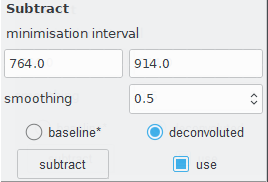
subtraction settings.
Clicking the subtract button runs the unmixing algorithm and results are plotted in green. If you’re happy with the results, click the use tickbox to
to continue using the unmixed spectrum in the interpolation and/or baseline correction tools.
subtraction of interference.
Deconvolution
deconvolve() is used for (optional) interference deconvolution, see its documentation for a comprehensive description
of all its parameters.

Deconvolution of an olivine spectrum.
The deconvolution algorithm first makes initial guesses for the positions of the convoluted peaks. The spectrum is then split into multiple deconvolution regions based on the initial guesses. More detailed estimates for convoluted peaks are made per region and more peaks are added iteratively if needed. Iterations are stopped once the residual of the baseline corrected and deconvoluted signals falls below a set threshold value, or when a maximum number of iterations is reached. Deconvolution results for all regions are merged to create the full deconvoluted spectrum.
Start deconvolutions by clicking the deconvolve button in the settings bar. Calculations may take several seconds and once they are finished deconvolved peaks are plotted in grey and the total deconvolved signal in blue.
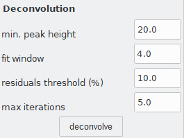
SilicH2O uses default values for some of deconvolution parameters, but the following have to be set by the user:
min. peak height
Minimum absolute peak height of the initally guessed peaks. When this value is too low, too many peaks will be fitted and calculations will be very slow. If this value is too high, some peaks will be skipped by the deconvolution. You can read which value is appropriate from the Y-axis of the interference plot: find the lowest peak you want fitted and check what its (baseline corrected) height is. Choose a value slightly lower than this.
Missed peaks with too low min. peak height.
fit window
fit window sets the width of the individual deconvolution regions. Widths are calculated as fit_window 
full width of the guessed peak and when deconvolution regions overlap they are merged.
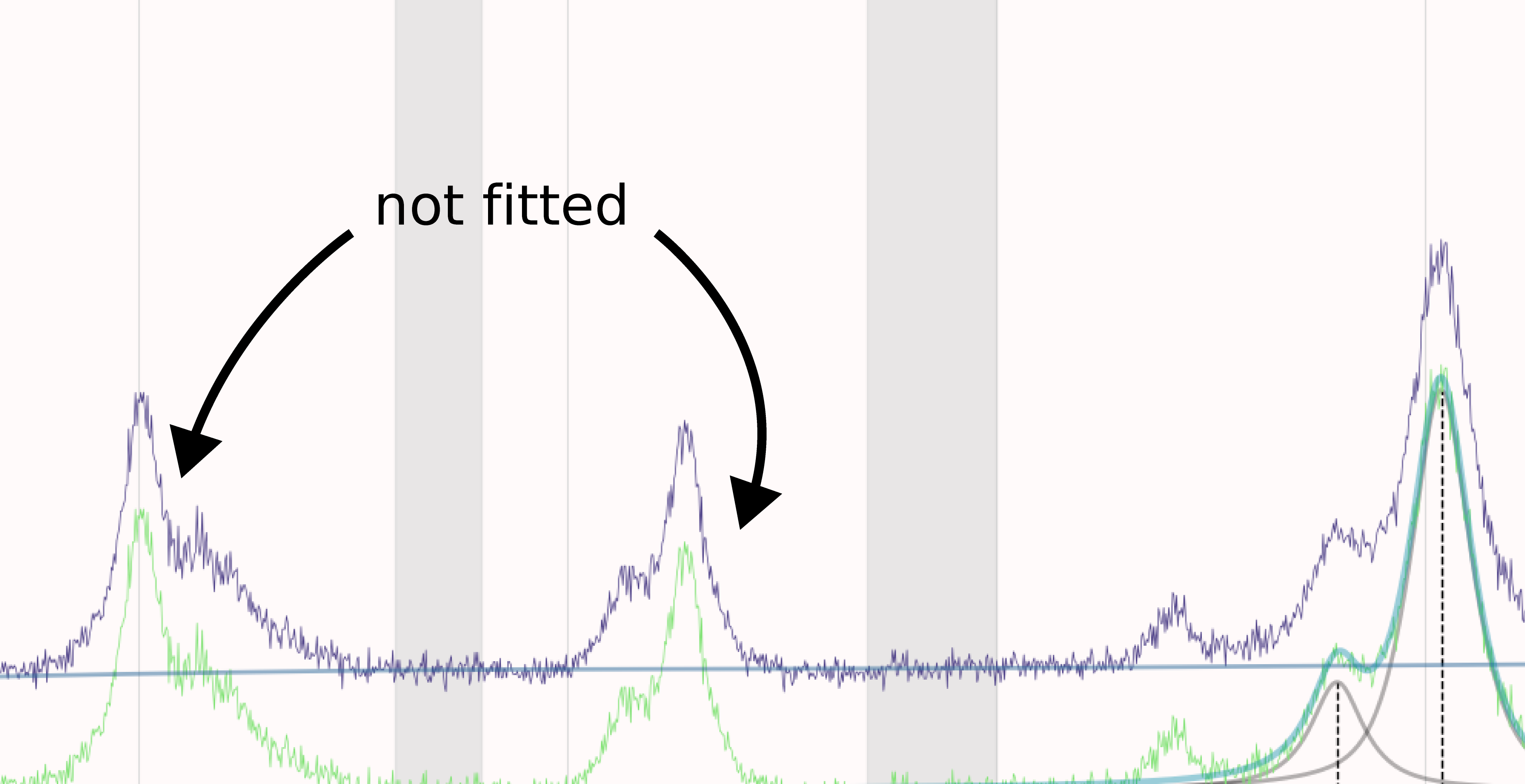
If fit window is set too high calculations become slow and deconvolution fits poor, especially for minor peaks. When its value is set too low, shoulder peaks might be missed.
If two peaks actually overlap, but fit window is not set sufficiently high for them to be in the same deconvolution region, the total deconvoluted signal may also overestimate the real signal.
This happens when overlapping tails from two adjacent deconvolution regions are added together when merging the full deconvoluted spectrum.
Values of 4–6 give good results for olivine.
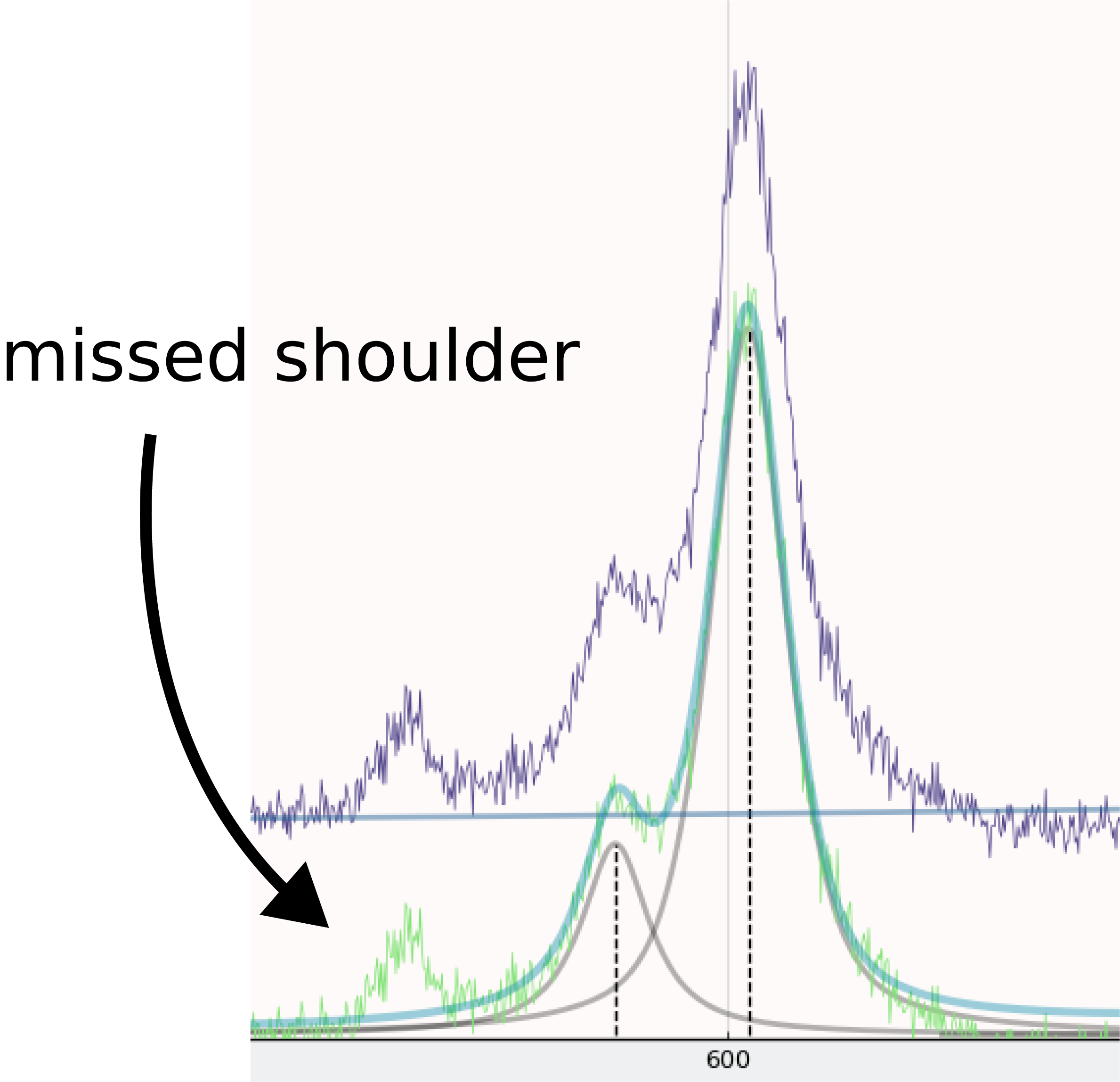
Missed shoulder with too low fit window.
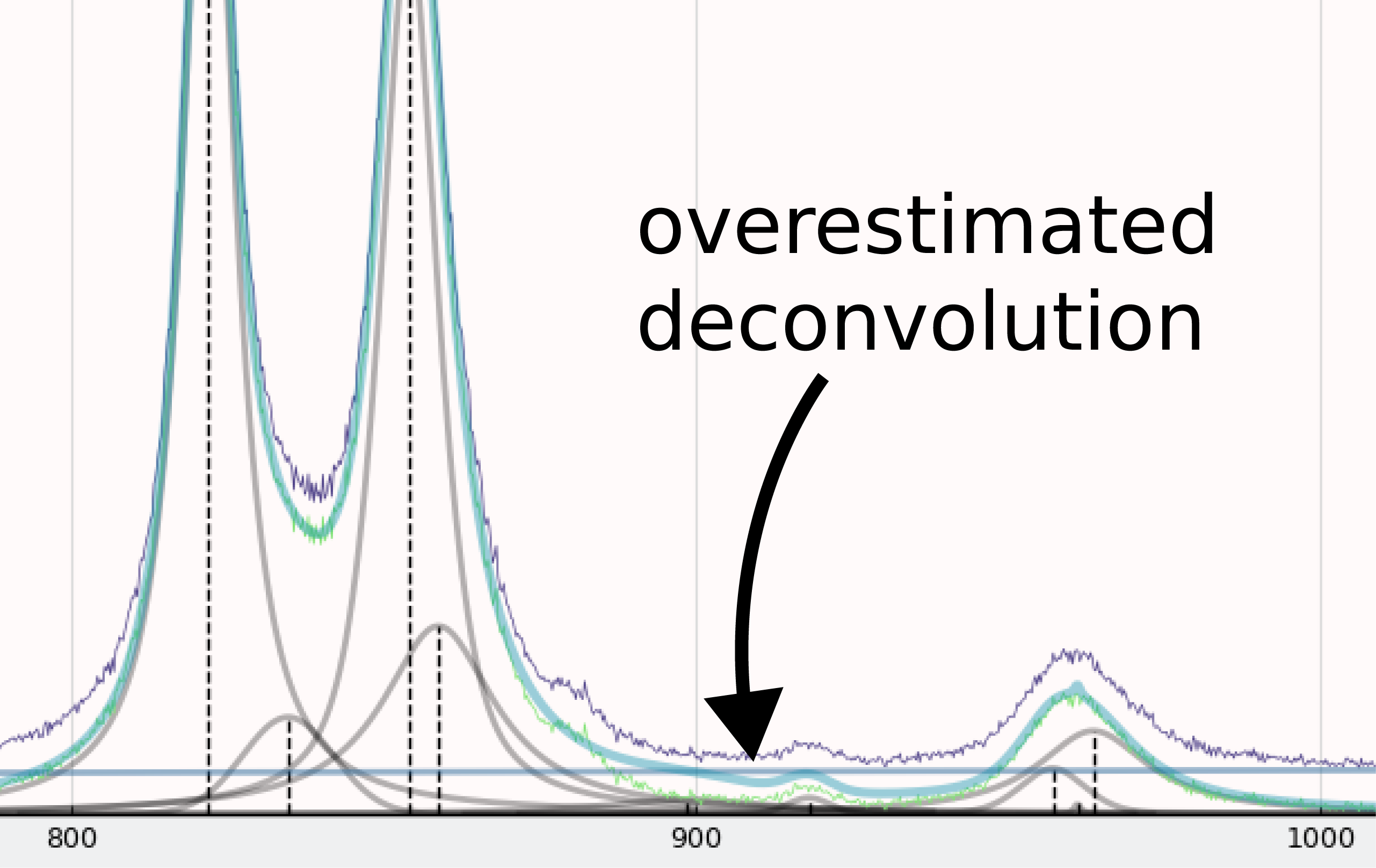
Overestimated deconvolution with too low fit window.
residuals threshold
fit iterations are stopped when the root-mean squared error of the deconvolution and baseline corrected signal has decreased less than residuals_threshold% compared to the previous iteration.
If this value is too high the deconvolution will have a poor fit and if its too low calculations take longer as more iterations are performed.
Values of 5–15% usually give good results

Poor deconvolution fit with too high residuals threshold or too low max iterations.
max iterations
The maximum number of iterations performed per deconvolution region. Together with residuals threshold it determines how many additional peaks will be added to each deconvolution region.
Too high values slow down calculations and overfit data, while too low values give poor deconvolution fits.
Values of ca. 5 give good results for olivine.