H2O calibration
The calibration window is opened from the Calibrate menu. In this window new calibrations can be made with the results from the active project, or existing calibrations can be imported and linked to the current project. The menu structure is explained on the getting started page.
Creating calibrations
After importing results from the active project via the menu Import → current project, all samples are listed in rows with data for  and reference H2O contents in columns.
H2O contents have to be set by the user by typing values in the appropriate cells. For each sample, you have to indicate wether to include the sample in the calibration
by clicking their respective
and reference H2O contents in columns.
H2O contents have to be set by the user by typing values in the appropriate cells. For each sample, you have to indicate wether to include the sample in the calibration
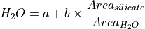
by clicking their respective use tickboxes. The calibration curve is updated in real-time and is calculated from
a linear regression of against H2O, as:
Results are plotted in real-time, where hovering over symbols shows the sample name. R2, p-value and standard error of estimate (SEE) statistics are also recalculated continuously and displayed in the top right window corner, together with the fitted intercept and slope.
New calibrations are saved via the menu File → save as. This saves the calibration data in a .cH2O file and all underlying spectral data in a new project file (in the .\calibration and .\calibration\projects folders respectively). Saving to the activate calibration is done via the menu File → save or with the Ctrl+s keyboard shortcut. .cH2O files can be exchanged between users, but make sure to only apply calibrations to spectra from the same Raman instrument.
Setting up a new H2O calibration.
Applying calibrations
Calibrations are linked to existing projects by importing their .cH2O file via the menu Import → from file.
They are applied to the active project by clicking the use tickbox below the regression statistics.
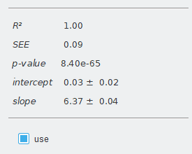
Regression statistics.